2D functions

Using their 1D analog as a starting point, you will implement the following 2D functions

• function y = myconv2D(fcol,frow,x) will perform a 2D convolution on the image x using the filter fcol on the columns and frow on the rows. Use the conv2 Maltlab routine. You will have to transpose one of the filters.
• function y = zeroinsert2D(x) inserts a column of zeros between every two columns of the image x, and acts similarly on the rows. The resulting image is roughly 4 times bigger than the original.
• function z = subsample2D(x) removes the columns and rows of the image x which have even indices. Follow carefully what is done in 1D to avoid errors
• function y = addSignals2D(u,v) which adds two images u and v. Be careful to follow the 1-D example and adapt it to matrices, since it is rather tricky.
• function WT = WaveTransform2D(u,h,g,scale) will perform the 2D wavelet transform on the image object u with the low pass filter h and the band pass filter g for a number of scales scale. Do not forget that three combinations of filters are used to compute the three detail images at each scale.
• function u = InvWaveTransform2D(WT,rh,rg,scale) will perform the inverse 2D wavelet transform on the image object u with the low pass reconstruction filter rh and the band pass reconstruction filter rg for a number of scales scale. The output is an image object.

These functions are not very difficult to write if you have their 1-D counterparts. This why no solution is provided here.
To check the coding of the function, perform a wavelet transform with the filter in Daub4.mat, compute its inverse transform, trim the output using the rd and cd delay fields as well as the dimensions of the original image, and display the difference between the original and the reconstructed image.

Here is, on the Y channel of the Lena image, the value of WT.Details{1}.r.s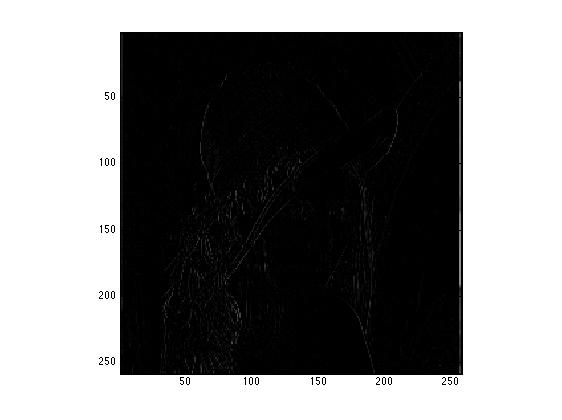

It is very dark, meaning that the details have little amplitude. Here is the same image with rescaled colormap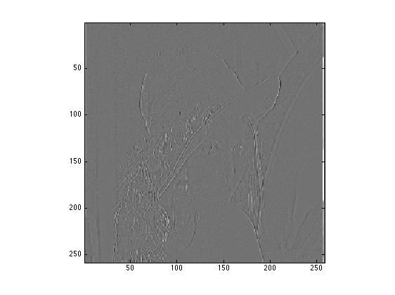

You can see the vertical edges of the image; this is because the band pass filters acts on the rows. As a consequence, its output is high when there is a locally strong variation in luminance; this corresponds to the vertical boundary of an object in the image.